n October 2025, the Institut de l’énergie Trottier published a report by Éloïse Edom and Normand Mousseau on an integrated definition of electricity peak demand in cold-climate regions, using Québec as the case study. (See https://iet.polymtl.ca/publications/rapport/definition-integree-pointe)

I know Normand Mousseau, so I read the report with interest. I find it useful on one very specific point: it helps clarify what Québec’s winter peak really is.

The topic may sound technical. It is not only technical.

In a power system like Québec’s, the winter peak is a structural constraint. The grid is designed around it. Supply contracts, transmission and distribution capacity, demand-response programmes, tariffs and a large share of investments are organized around a few hours, or a few days, when the system is under heavy stress.

The report’s main contribution is that it shifts the discussion.

We often talk about the peak as a moment: the highest hour of the year. The report instead proposes looking at it as a phenomenon that unfolds over time, with power, duration, energy to be shifted and a period of accumulation before the peak event.

That is, in my view, the most interesting contribution of the document.

(LinkedIn: https://www.linkedin.com/pulse/winter-peak-flexibility-problem-long-duration-storage-benoit-marcoux-p9iye/)

A Method for Thinking About the Peak Over Time

The method deserves to be explained simply, because it is not obvious on first reading.

For a given window, for example 36 or 72 hours around the annual peak, the method asks how far maximum demand could be lowered if the excess energy above a new ceiling were accumulated before the peak event, then returned during the peak.

The authors start with the hourly electricity demand curve, the 8,760 hours of the year. They then calculate an average power level, called a “power ceiling”, for different time windows before the peak: 12 hours, 36 hours, 72 hours, 96 hours, and so on.

When actual demand exceeds that ceiling, there is a peak event.

The energy to be shifted is the area between the actual demand curve and the power ceiling. So, it is not the full consumption over the period that needs to be shifted. It is only the portion above the ceiling.

The report then identifies the critical peak event, meaning the one where that area is the largest. That is the event requiring the most energy to be shifted.

Finally, the authors calculate how long it would have taken to accumulate that energy before the peak. They assume that accumulation occurs in the hours immediately before the event, that the system is initially empty, and that there are no losses.

This assumption of charging immediately before the peak matters. The duration of accumulation does not depend only on the energy to be shifted. It also depends on the demand profile before the peak. If the grid is already heavily loaded before the event, there is less room to charge. If demand is lower, there is more room.

That is what makes the approach interesting. It does not look only at the peak itself. It also looks at what happens before it.

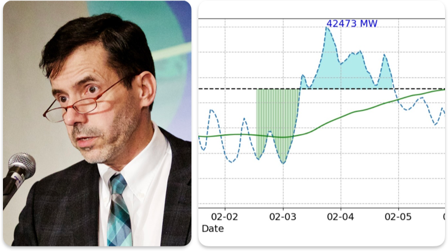
The chart above illustrates the logic well. The dotted blue curve shows historical demand, peaking at 42.5 GW. The green curve shows the 72-hour moving average. The black dotted line gives the corresponding ceiling, here around 36.3 GW. The blue area above the ceiling represents the energy to be smoothed during the peak event. The green area before the peak represents the energy to be accumulated ahead of it.

It is this relationship between the dip before the event and the excess during the peak that gives the approach its operational value.

What the Orders of Magnitude Show

During the two winters studied, Québec’s annual system peak was around 40 to 42 GW.

In that context, a 36-hour window would already lower the peak by about 3.5 to 3.9 GW, while shifting about 13 to 15 GWh of energy. That is close to one tenth of the annual peak.

With a 72-hour window, the reduction would increase to about 5.2 to 6.1 GW, with about 40 to 97 GWh to shift, depending on the winter studied. That is roughly one seventh of the annual peak.

Those numbers can look huge. They look less so when compared with recent battery deployments elsewhere.

California has already installed more than 20 GW of battery storage, including residential, commercial and grid-scale systems. In the CAISO market, grid-connected batteries now represent several dozen GWh. Texas has also exceeded 10 GW of grid-connected batteries, with more than 20 GWh of energy capacity. In Europe, total battery storage capacity is now measured in dozens of GWh. In Australia, the National Electricity Market added more than 4 GW and more than 10 GWh of grid-scale batteries in only twelve months.

The comparison is not perfect. These grids do not manage the same peak, the same climate, or the same demand structure. But it gives an order of magnitude: a few GW and a couple of dozen GWh are no longer extravagant figures in a modern electricity system.

Nor should we imagine that all this capacity would have to come from large grid-scale batteries owned by the distributor or by a producer. Some can be connected to the transmission or distribution network. Some can be behind the meter, at residential, commercial or industrial customer sites, provided it is aggregated, controllable and properly compensated.

This value is not limited to peak management. Distributed batteries can also contribute to resilience during outages. As electricity becomes, for many households, the only final energy source, reducing the impact of service interruptions becomes much more concrete than it used to be.

Australia illustrates this point well. Behind-the-meter batteries can matter. Residential batteries installed in 2025 already represent several GWh of capacity, and South Australia alone now has more than one GWh of residential batteries.

For peak management, the location of batteries also matters as much as their technology. Capacity placed near a distribution constraint, or behind the meter in selected buildings, can be more valuable than equivalent capacity located elsewhere on the grid.

This logic can also change how new buildings are designed. Instead of sizing each building as though it could draw as much power as it wants from the grid without constraint, we could impose or encourage a maximum demand limit while maintaining the same level of comfort. That would push toward better choices in building envelope, heating, thermal storage, batteries, controls and local demand management.

72 Hours of Analysis Does Not Mean 72 Hours of Storage

This is where an important distinction must be made.

A 72-hour analytical window does not mean that a storage system must be able to deliver its full power for 72 hours.

The 72-hour window is used to understand the peak phenomenon in its meteorological and operational context: the arrival of cold weather, the rise in demand, the peak itself and then the return to a more normal level.

The storage system, for its part, must mainly be able to shift the excess energy above a given power ceiling.

So, the starting point must be the area above the ceiling. That area gives the MWh to be shifted. The MW then indicate the power needed to shave the peak, hour by hour. Both dimensions are essential, but they do not answer the same question.

This distinction avoids a common mistake: thinking in terms of “battery hours” before looking at the energy to be shifted.

For the winter peak, the right question is not: how many hours of battery do we need?

The right question is: how many MWh need to be available, at what time, and with how many MW to respect the target ceiling?

The C-Rate: Useful, But It Has to Be Used Carefully

Once we have separated the two questions, the MWh to be shifted and the MW needed to shave the peak, we can use the C-rate to translate this into battery-system language.

The C-rate simply expresses the ratio between output power and energy capacity:

C = MW/MWh

A system with C = 0.5 corresponds to 2 MWh per MW of power. This is often called, as shorthand, a “2-hour” system.

A system with C = 0.25 corresponds to 4 MWh per MW of power, or a “4-hour” system. That is now a very common configuration for grid-scale batteries. In Texas, 2-hour systems are also very common, while 4-hour systems are becoming more widely deployed.

A system with C = 0.125 corresponds to 8 MWh per MW. These configurations exist in techno-economic analysis, but they are much less common in current lithium-ion battery deployments. Configurations at C = 0.25 or C = 0.5 generally provide more versatility, with the additional power cost often justified by the extra services they can provide.

But the language matters.

Saying that a system is “4-hour” does not mean it must be discharged in four hours. It means it can provide full power for four hours.

It can be discharged more slowly, over a longer period, at lower power. Its output can also vary hour by hour depending on the peak-shaving need, like the blue area in the example: higher at the top of the peak, lower on the shoulders.

But it cannot deliver all its energy in less than four hours without a larger power chain, including a more powerful inverter.

This distinction also matters for costs.

For a given energy capacity, a system with more MW generally costs more because it requires a stronger power chain: inverters, transformers, protection systems and interconnections. For a given power level, a system with more MWh generally costs more because it requires more cells, modules, containers, thermal management and safety systems.

In other words, MW and MWh do not have the same cost structure.

What the Data Suggest for Batteries

Using the report’s data, we can calculate the implied power-to-energy ratio of the storage system required to shave the critical peak.

For 12- and 36-hour windows, the results are close to common grid-scale battery configurations. Depending on the winter studied, the energy equivalent is about 2.6 to 4.4 MWh per MW of power. That is in the range of so-called 4-hour systems.

For a 72-hour window, the picture changes. The energy equivalent reaches about 7.6 MWh per MW for winter 2021–2022, but nearly 16 MWh per MW for winter 2022–2023. For 96 hours, it is about 8 MWh per MW in one case, but more than 20 MWh per MW in the other.

These ratios do not mean that systems must necessarily be built with these exact C-rates. They indicate the relationship between the power to be shaved and the energy to be shifted for the events analyzed.

If we use batteries typical of current grid-scale deployments, for example 2- or 4-hour systems, the MW capacity could be higher than what is strictly required for this winter peak-shaving use case. That extra power capacity is not necessarily wasted. It can serve other uses: fast response, ancillary services, arbitrage, local congestion relief, or distribution support.

But for a 72-hour window, the central issue remains available energy capacity. There must be enough MWh to cover the area above the ceiling. Only after that comes the question of how many MW to install and what value any excess MW can provide for other services.

Two mistakes should, therefore, be avoided.

The first would be to conclude that a phenomenon analyzed over 72 hours requires 72 hours of storage. That is not what the data show.

The second would be to conclude that batteries must be operated on a short, repetitive cycle, as though they necessarily had to charge and discharge once or twice a day. That is not the right frame here. For the winter peak, charge and discharge need to be planned over a longer horizon, based on the arrival of cold weather, the demand profile before the peak and the energy to be shifted above the ceiling.

This kind of smoothing can also reduce start-stop cycles for turbine-generator units, limiting mechanical wear and improving the operation of the existing fleet.

The Economic Point: Avoided MW Versus Added MWh

This reading opens an important economic question: what is the right balance between avoided peak MW and added storage MWh?

On the grid side, costs are mostly tied to the MW that must be served or avoided: generation, supply, transmission, distribution, capacity margins and demand-response programmes. In Hydro Québec‘s context, the calculation is more complex, because the value of avoided MW also depends on interruptible-power contracts and other peak-management tools.

On the battery side, costs are split between power and energy. At a given power level, adding MWh mainly means adding cells, modules, thermal management and safety systems. In the current cost structure, the total cost is generally more sensitive to MWh, meaning the blue area to cover, than to maximum MW.

The Tomago project in Australia gives a useful benchmark: 500 MW and 2,000 MWh, a 4-hour battery, at an announced cost of about 800 million Australian dollars. Since the Australian and Canadian dollars are close to parity, this gives an order of magnitude of about 1.6 million Canadian dollars per MW, or about 400,000 Canadian dollars per MWh.

Applied mechanically to the needs identified in the report, this would mean about 5 to 6 billion dollars to shift the 13 to 15 GWh associated with the 36-hour window. For the 72-hour window, with 40 to 97 GWh to shift depending on the winter, the order of magnitude would be more like 16 to 39 billion dollars.

These are large amounts. But they should not be read as the cost of a single solution made entirely of batteries. They provide a benchmark for comparing the required MWh with the cost of the infrastructure that would otherwise be needed to serve the peak.

The comparison with Hydro-Québec is instructive. The report notes that Hydro-Québec’s avoided capacity costs are in the range of $164 to $249 per kW-year, depending on whether the additional kW requires transmission and distribution additions. Applied to the peak reductions in the report, this represents about $0.6 to $1.0 billion per year for a 36-hour window, and about $0.9 to $1.5 billion per year for a 72-hour window.

A very simple comparison of these annual values with the battery-cost estimates inspired by Tomago gives a rough payback period of about 5 to 10 years for the 36-hour window. For the 72-hour window, the range becomes much wider, from roughly 11 to more than 40 years, confirming that the economic optimum is not obvious and depends heavily on the energy to be shifted.

We can also compare this with Churchill Falls Extension future hydrogeneration station. That project would add about 1,100 MW of capacity for an estimated cost of $4.6 billion, including financing, or around $4.2 million per MW. This is not directly comparable with batteries: hydropower provides capacity backed by an existing reservoir and has a very long life. Still, the order of magnitude shows that battery-based flexibility, especially for windows such as 36 hours, deserves to be assessed seriously against new centralized peak resources.

This is not proof of profitability. Battery costs would have to be annualized, and the analysis would have to account for service life, degradation, charging costs, location and the value of other services provided. But the comparison is enough to show that the calculation should be done seriously.

And it is worth remembering why Tomago is interesting: these costs are possible in a market where the ecosystem for developing, procuring, building, interconnecting and operating batteries is already effective. The cost of a battery, therefore, does not depend only on the technology. It also depends on the maturity of the ecosystem that deploys it.

There is probably an optimal point between avoided peak MW and added storage MWh. That optimum is not fixed. It changes with battery costs, avoided grid-infrastructure costs, interruptible-power contract conditions, the location of constraints, the actual shape of the peak and the value of other services that storage can provide.

Québec Is in a Particular Position

The report focuses on Québec’s winter peak. This context is specific: high electrification of heating, a dominant hydropower fleet, an annual peak concentrated around cold snaps and a strong ability by Hydro-Québec to operate the system.

This is not the same problem as a Dunkelflaute event in Northern Europe or around the Baltic Sea, where the challenge comes from low wind and solar generation over several days. In that case, the need can truly become a long-duration storage or supply problem.

Québec is especially privileged. Its hydropower fleet already provides a form of very large-scale seasonal storage that many grids would envy. Several are still trying to build, or replace, such capability with much more expensive solutions.

Batteries should therefore not be seen as a substitute for this seasonal storage. They can instead complement it by adding short- and medium-duration flexibility where the hydropower system, the grid or demand-response programmes reach their operational limits.

This does not mean the approach applies only to Québec. It could become relevant in other northern regions that are rapidly electrifying heating and vehicles, including Ontario, the U.S. Northeast and some Nordic countries.

These regions may also want to avoid building infrastructure capable of delivering several GW for only a few hours of extreme cold. The difference with a European Dunkelflaute matters: here we are talking about a sharp peak, often cold-related, not a prolonged renewable-generation shortfall lasting several days.

This evolution could even strengthen Québec’s strategic value.

If neighbouring grids also electrify their heating, cold-weather peaks are likely to become more synchronized. In that context, relying on imports during critical hours will become less reliable and more expensive. Québec therefore has an interest in developing its own flexibility, but also in becoming a leader in managing this type of peak.

This is where the IET report opens a useful path.

It shows that Québec’s winter peak is not primarily an annual-energy problem. It is a problem of power, timing and synchronization. The energy above the peak ceiling remains small relative to annual consumption, but it is concentrated at the moment when the grid is most constrained.

The Real Conclusion

The conclusion for Québec is not: “Batteries solve every storage problem.”

It is more precise than that.

For Québec’s winter peak, 36- or 72-hour windows can be useful analytical frames without implying a need for storage of the same duration.

The data point instead to a need for modular flexibility: enough MWh to cover the area above the ceiling, enough MW to shave the peak, and probably a portfolio combining batteries, thermal storage, demand response and demand control.

That nuance matters.

It moves the discussion away from an abstract debate about long-duration storage and toward a much more concrete discussion about the sizing of flexibility resources, their cost, their location, their operation and their system value.

The next step would be to translate this approach into real deployment scenarios.

Where should storage systems be located?

How many MWh need to be available?

How many MW are actually needed?

What share can come from the grid, and what share can come from behind-the-meter resources?

For which combined services?

And with what avoided value for the grid?

That is where the discussion becomes genuinely strategic for Hydro-Québec and for Québec.